nlcpy.random.Generator.normal
- Generator.normal(self, loc=0.0, scale=1.0, size=None)
Draws random samples from a normal (Gaussian) distribution.
The probability density function of the normal distribution, first derived by De Moivre and 200 years later by both Gauss and Laplace independently, is often called the bell curve because of its characteristic shape (see the example below).
The normal distributions occurs often in nature. For example, it describes the commonly occurring distribution of samples influenced by a large number of tiny, random disturbances, each with its own unique distribution.
- Parameters
- locfloat
Mean ("centre") of the distribution.
- scalefloat
Standard deviation (spread or "width") of the distribution. Must be non-negative.
- sizeint or tuple of ints, optional
Output shape. If the given shape is, e.g.,
(m, n, k), thenm * n * ksamples are drawn.
- Returns
- outndarray
Drawn samples from the parameterized normal distribution.
注釈
The probability density for the Gaussian distribution is
where
is the mean and
the standard deviation. The square of the standard deviation,
, is called the variance.
The function has its peak at the mean, and its "spread" increases with the standard deviation (the function reaches 0.607 times its maximum at
and
).
制限事項
If loc is neither a scalar nor None : NotImplementedError occurs.
If scale is neither a scalar nor None : NotImplementedError occurs.
Examples
Draw samples from the distribution:
>>> import nlcpy as vp
>>> mu, sigma = 0, 0.1 # mean and standard deviation
>>> s = vp.random.default_rng().normal(mu, sigma, 1000)
Verify the mean and the variance:
>>> abs(mu - vp.mean(s))
array(0.00206415)  # may vary
>>> abs(sigma - vp.std(s, ddof=1))
array(0.00133596)  # may vary
Two-by-four array of samples from N(3, 6.25):
>>> vp.random.default_rng().normal(3, 2.5, size=(2, 4))
array([[-4.49401501,  4.00950034, -1.81814867,  7.29718677],   # random
       [ 0.39924804,  4.68456316,  4.99394529,  4.84057254]])  # random
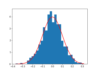
Display the histogram of the samples, along with the probability density function:
>>> import matplotlib.pyplot as plt
>>> count, bins, ignored = plt.hist(s.get(), 30, density=True)
>>> plt.plot(bins, 1/(sigma * vp.sqrt(2 * vp.pi)) *
...                vp.exp( - (bins - mu)**2 / (2 * sigma**2) ),
...          linewidth=2, color='r')
...
>>> plt.show()

Two-by-four array of samples from N(3, 6.25):
>>> vp.random.default_rng().normal(3, 2.5, size=(2, 4))
array([[ 1.53904187,  3.36100709, 11.21828966,  6.85936673],  # random
       [ 1.50665756,  5.35682791,  4.66053878,  3.55770521]]) # random